本章节主要在讨论一些技术来解决协作问题。这些协助技术被称之为 stochastic optimization (随机优化)
这章代码的勘误比较多,可以参考文中注释
组团旅游 #
书中定义了一个组团旅游的场景。
为来自不同地方去往同一地点的人们安排一次旅游是一件极富挑战性的事情。 要求:家庭成员来自全国各地,他们希望在纽约会面。他们将在同一天到达,并在同一天离开,而且他们想搭乘相同的交通工具往返飞机场。 每天有许多航班从任何一位家庭成员的所在地飞往纽约,飞机起飞时间是不同的,价格和续航时间上也都不尽相同。
基础定义
# 人员
people = [('Seymour','BOS'),
          ('Franny','DAL'),
          ('Zooey','CAK'),
          ('Walt','MIA'),
          ('Buddy','ORD'),
          ('Les','OMA')]
# 目的地
destination='LGA'
飞行清单
flights={}
#
for line in file('schedule.txt'):
  origin,dest,depart,arrive,price=line.strip().split(',')
  flights.setdefault((origin,dest),[])

  # Add details to the list of possible flights
  flights[(origin,dest)].append((depart,arrive,int(price)))
打印调度表
def printschedule(r):
  for d in range(len(r)/2):
    name=people[d][0]
    origin=people[d][1]
    out=flights[(origin,destination)][int(r[d])]
    ret=flights[(destination,origin)][int(r[d+1])] # 原文应该错了,应该是 r[2*d+1]
    print '%10s%10s %5s-%5s $%3s %5s-%5s $%3s' % (name,origin,
                                                  out[0],out[1],out[2],
                                                  ret[0],ret[1],ret[2])
这样就可以打印出来如下
  s = [1, 4, 3, 2, 7, 3, 6, 3, 2, 4, 5, 3]
  printschedule(s)

   Seymour       BOS  8:04-10:11 $ 95 12:08-14:05 $142
    Franny       DAL 12:19-15:25 $342 10:51-14:16 $256
     Zooey       CAK 10:53-13:36 $189  9:58-12:56 $249
      Walt       MIA  9:15-12:29 $225 16:50-19:26 $304
     Buddy       ORD 16:43-19:00 $246 10:33-13:11 $132
       Les       OMA 11:08-13:07 $175 15:07-17:21 $129
准备好这些基础的就开始核心部分了
成本函数 #
def schedulecost(sol):
  totalprice=0
  latestarrival=0
  earliestdep=24*60

  for d in range(len(sol)/2):
    # 往返航班的航班
    origin=people[d][1]
    outbound=flights[(origin,destination)][int(sol[d])]
    returnf=flights[(destination,origin)][int(sol[2*d+1])]

    # 往返航班总价
    totalprice+=outbound[2]
    totalprice+=returnf[2]

    # 循环的时候,刚好记录下最早和最晚的时间
    if latestarrival<getminutes(outbound[1]): latestarrival=getminutes(outbound[1])
    if earliestdep>getminutes(returnf[0]): earliestdep=getminutes(returnf[0])

  # 因为每个人都需要等待人齐,这里就计算了等待时间
  totalwait=0
  for d in range(len(sol)/2):
    origin=people[d][1]
    outbound=flights[(origin,destination)][int(sol[d])]
    returnf=flights[(destination,origin)][int(sol[d+1])]
    totalwait+=latestarrival-getminutes(outbound[1])
    totalwait+=getminutes(returnf[0])-earliestdep

  # 如果换车要多付一天就+50
  if latestarrival>earliestdep: totalprice+=50

  return totalprice+totalwait
Random 随机搜索 #
最近的解法就是尝试随机解答,然后比较它们的成本。找到一个最低成本解。
def randomoptimize(domain,costf):
  best=999999999
  bestr=None
  for i in range(0,1000):
    # 创建一个随机解
    r=[float(random.randint(domain[i][0],domain[i][1]))
       for i in range(len(domain))]

    # 计算成本
    cost=costf(r)

    # 和最好的比较
    if cost<best:
      best=cost
      bestr=r
  return bestr
大力出奇迹的办法
# 输入是一个人和他的所有航班 [(0,8),(0,8), ....]
s = randomoptimize(domain=[(0,8)]*(len(people)*2),costf=schedulecost)
print schedulecost(s)
printschedule(s)
2932
  Seymour       BOS 11:16-13:29 $ 83 10:33-12:03 $ 74
  Franny       DAL 10:30-14:57 $290 10:51-14:16 $256
    Zooey       CAK 12:08-14:59 $149 12:01-13:41 $267
    Walt       MIA 11:28-14:40 $248 12:37-15:05 $170
    Buddy       ORD 12:44-14:17 $134 17:06-20:00 $ 95
      Les       OMA 12:18-14:56 $172 18:25-20:34 $205
Hill Climbing 爬山法 #
随机显然是一个特别低效的算法,如果变量范围很大,几乎不可能找到最优解。所以,我们需要一个更好的算法。
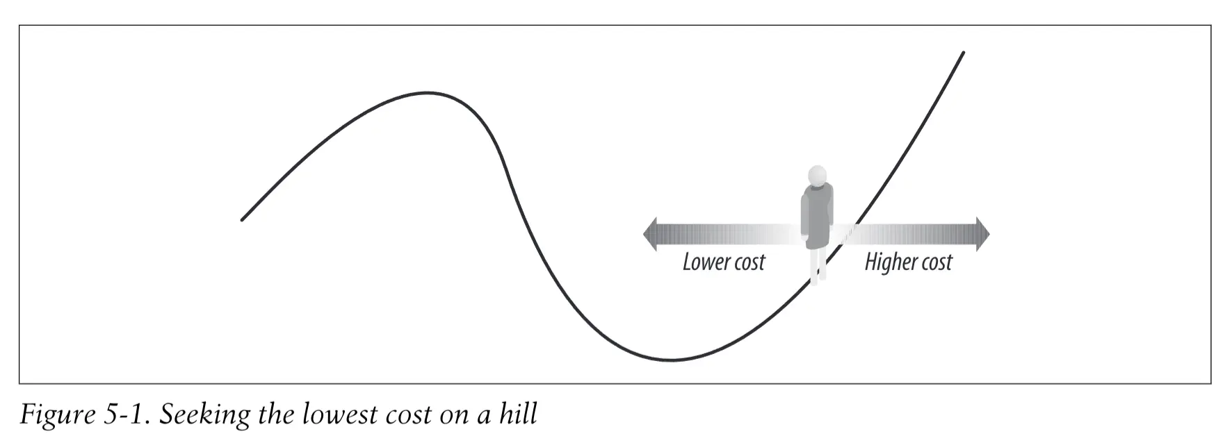
爬山法是从一个随机解开始,向周围的解尝试,然后选择成本最低的那个解作为下一次的解。
def hillclimb(domain,costf):
  # 首先随机生成一个解
  sol=[random.randint(domain[i][0],domain[i][1])
      for i in range(len(domain))]
  # 主循环,直到无法改进才退出
  while 1:
    # 申明一个相邻解
    neighbors=[]

    for j in range(len(domain)):
      # 前一一个航班偏移,或者向后一个航班偏移,记录下来
      if sol[j]>domain[j][0]:
        neighbors.append(sol[0:j]+[sol[j]-1]+sol[j+1:])
      if sol[j]<domain[j][1]:
        neighbors.append(sol[0:j]+[sol[j]+1]+sol[j+1:])

    # 算算现在的
    current=costf(sol)
    best=current
    # 计算相近的
    for j in range(len(neighbors)):
      cost=costf(neighbors[j])
      if cost<best:
        best=cost
        sol=neighbors[j]

    # 无法提高了就返回
    if best==current:
      break
  return sol
结果如下
s = hillclimb(domain=[(0,8)]*(len(people)*2),costf=schedulecost)
print schedulecost(s)
printschedule(s)

3094
   Seymour       BOS 13:40-15:37 $138 12:08-14:05 $142
    Franny       DAL 12:19-15:25 $342 12:20-16:34 $500
     Zooey       CAK 13:40-15:38 $137 12:01-13:41 $267
      Walt       MIA 12:05-15:30 $330 11:08-14:38 $262
     Buddy       ORD 12:44-14:17 $134 14:19-17:09 $190
       Les       OMA 12:18-14:56 $172  9:31-11:43 $210
但是爬山法显然有个明显的问题,可能被困在了局部最优解上。
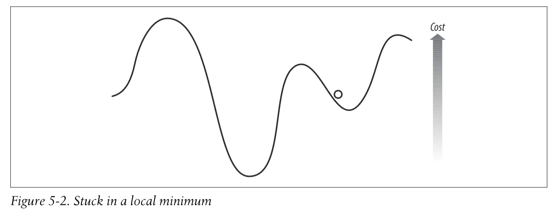
Simulated annealing 模拟退火 #
模拟退火算法:受物理学领域启发而来的一种优化算法。退火是指将合金加热后再慢慢冷却的过程。大量的原子因为受到激发而向周围跳跃,然后有逐渐稳定到一个低能阶的状态,所以这些原子能够找到一个低能阶的配置(configuration)
算法的关键部分在于: 如果新的成本值更低,则新的题解就会成为当前题解,这和爬山法非常相似。不过,如果成本值更高的话,则新的题解仍将可能成为当前题解,这是避免局部最小值问题的一种尝试。
较差解被接受的概率为
\(p=e^{(-(highcost-lowcost)/temperature)}\)模拟退火算法之所以管用,因为它在退火过程的开始阶段会接受变现较差的解。随着退火过程的不断进行,算法越来越不可能接受较差的解,直到最后,它只会接受更优的解。
def annealingoptimize(domain,costf,T=10000.0,cool=0.95,step=1):
  # 初始化一个随机解
  vec=[float(random.randint(domain[i][0],domain[i][1]))
       for i in range(len(domain))]

  while T>0.1:
    # 选择一个随机的下标索引
    i=random.randint(0,len(domain)-1)

    # 选择改变方向
    dir=random.randint(-step,step)

    # 创建一个新的答案
    vecb=vec[:]
    # i 项改变
    vecb[i]+=dir
    # 这个值要符合约束
    if vecb[i]<domain[i][0]: vecb[i]=domain[i][0]
    elif vecb[i]>domain[i][1]: vecb[i]=domain[i][1]

    # 计算新旧的值
    ea=costf(vec)
    eb=costf(vecb)
    # 决定是否接受新的解
    p=pow(math.e,-(eb-ea)/T)

    # 如果接受,并且概率上也接受
    if (eb<ea or random.random()<p):
      vec=vecb

    # 降温
    T=T*cool
  return vec
结果如下
s = annealingoptimize(domain=[(0,8)]*(len(people)*2),costf=schedulecost)
print schedulecost(s)
printschedule(s)

2789
   Seymour       BOS 12:34-15:02 $109 10:33-12:03 $ 74
    Franny       DAL 10:30-14:57 $290 10:51-14:16 $256
     Zooey       CAK 10:53-13:36 $189 10:32-13:16 $139
      Walt       MIA 11:28-14:40 $248 11:08-14:38 $262
     Buddy       ORD 12:44-14:17 $134 17:06-20:00 $ 95
       Les       OMA 11:08-13:07 $175  6:19- 8:13 $239
Genetic Algorithm 遗传算法 #
遗传算法:受自然科学的启发,运行过程是先随机生成一组解,称之为种群(population)。在优化过程的每一步,算法会计算整个种群的成本函数,从而得到一个有关题解的有序列表。 在对题解进行排序之后,一个新的种群
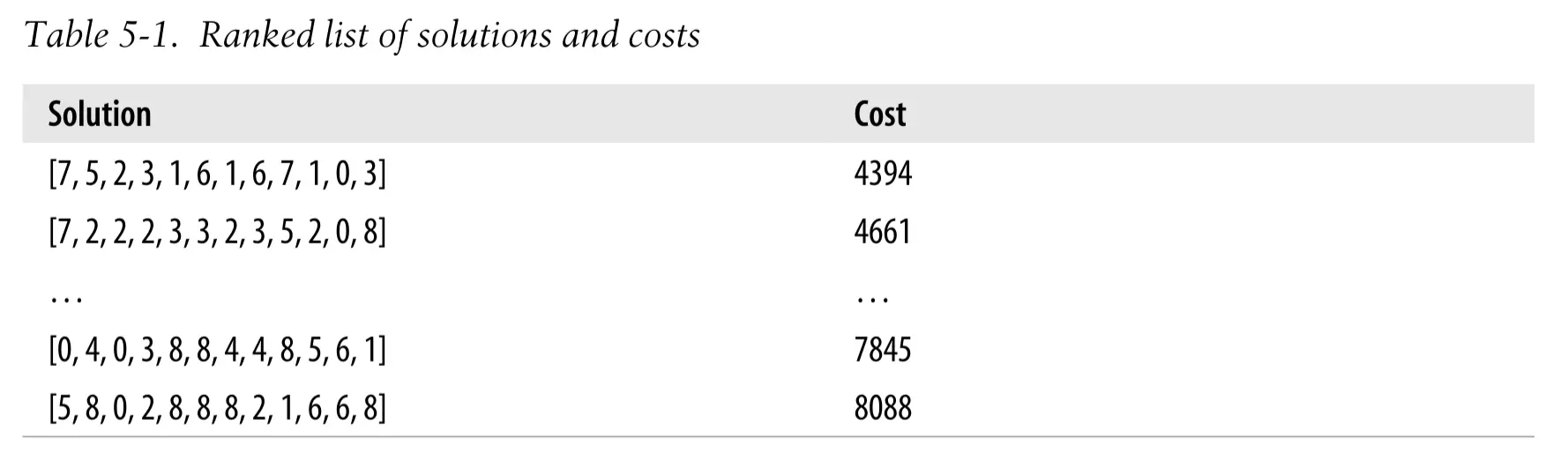
然后进行 精英选拔法(elitism):将但前种群中位于最顶端的题解加入其所在的新种群中。余下部分是有修改最优解后形成的全新解组成的。
两种修改题解的方法:
-
变异(mutation):对一个既有解进行微小的、简单的、随机的改变。
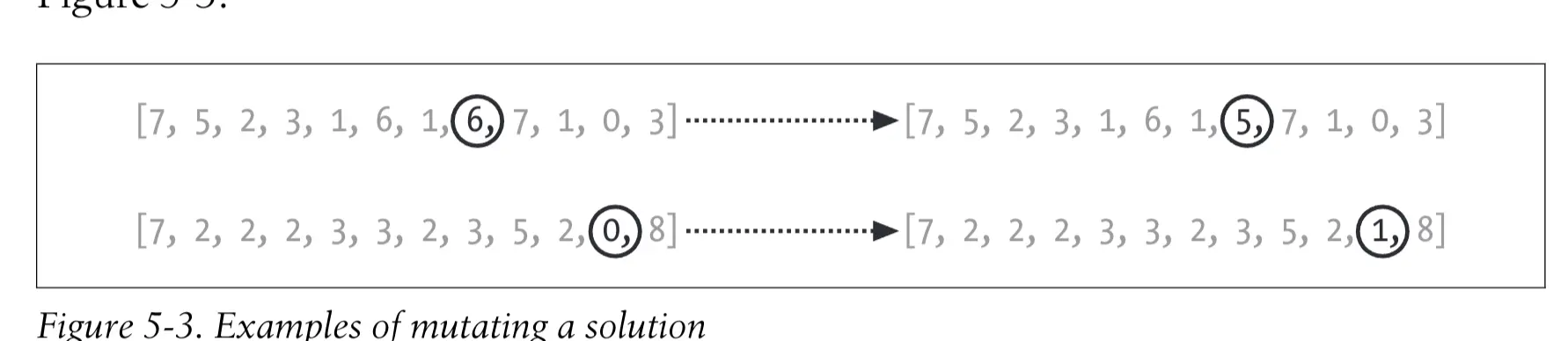
-
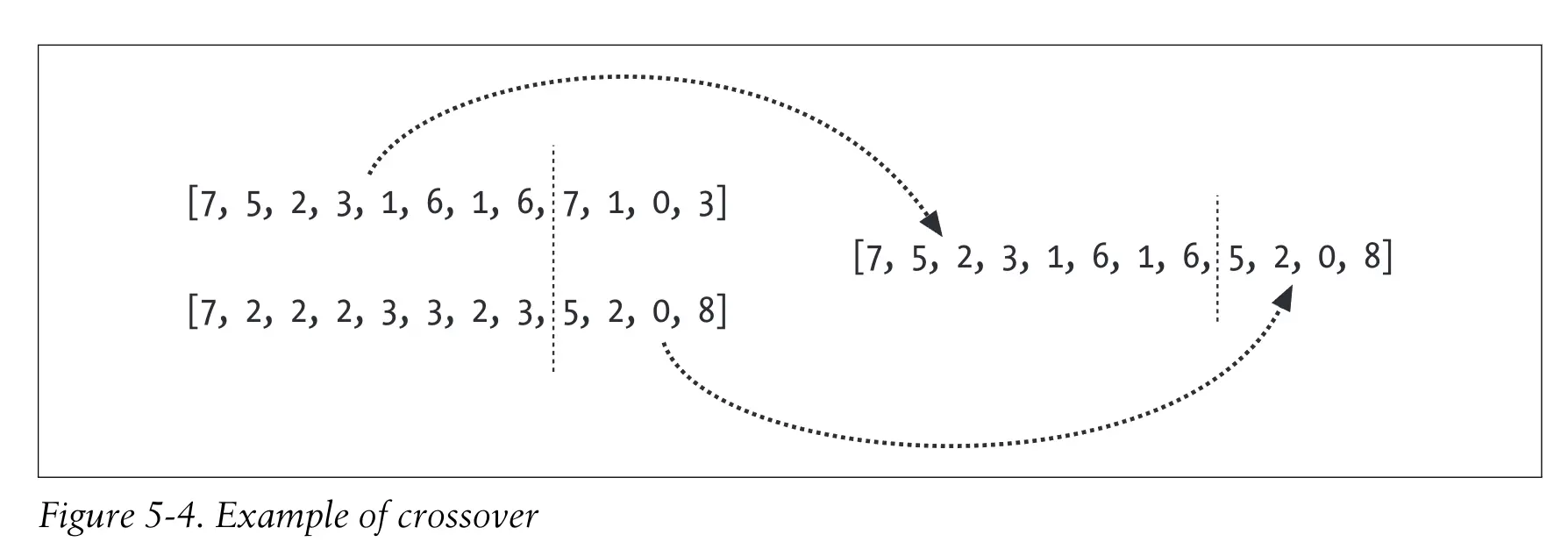
交叉(crossover)或配对(breeding):选取最有解中的两个解,然后将它们按某种方式进行结合。
一个新的种群是通过对最优解进行随机的变异和配对处理构造出来的,它的大小通常与旧的种群相同。尔后,这一过程会一直重复进行。达到指定的迭代次数,或者连续经过数代后题解都没有得到改善,整个过程就结束了。
def geneticoptimize(domain,costf,popsize=50,step=1,
                    mutprod=0.2,elite=0.2,maxiter=100):
  # 变异操作,随机找个点然后变异一下
  def mutate(vec):
    i=random.randint(0,len(domain)-1)
    if random.random()<0.5 and vec[i]>domain[i][0]:
      return vec[0:i]+[vec[i]-step]+vec[i+1:]
    elif vec[i]<domain[i][1]:
      return vec[0:i]+[vec[i]+step]+vec[i+1:]
    # 这里有个bug,有可能走到 elif 概率的时候 vec[i] >= domain[i][1] 这时候需要无法变异
    return vec

  # 交叉操作,随机找个点然后交叉
  def crossover(r1,r2):
    i=random.randint(1,len(domain)-2)
    return r1[0:i]+r2[i:]

  # 生成 popsize 的种群
  pop=[]
  for i in range(popsize):
    vec=[random.randint(domain[i][0],domain[i][1])
         for i in range(len(domain))]
    pop.append(vec)

  # 计算精英的数量
  topelite=int(elite*popsize)

  # 迭代N代
  for i in range(maxiter):
    scores=[(costf(v),v) for v in pop]
    scores.sort()
    ranked=[v for (s,v) in scores]

    # 计算出精英
    pop=ranked[0:topelite]

    # 增加各种的变异和交叉
    while len(pop)<popsize:
      # 按纪律进行变异或者交叉
      if random.random()<mutprob:

        # Mutation
        c=random.randint(0,topelite)
        pop.append(mutate(ranked[c]))
      else:

        # Crossover
        c1=random.randint(0,topelite)
        c2=random.randint(0,topelite)
        pop.append(crossover(ranked[c1],ranked[c2]))

    # Print current best score
    print scores[0][0]

  return scores[0][1]
结果是
s = geneticoptimize(domain=[(0,8)]*(len(people)*2),costf=schedulecost)
print schedulecost(s)
printschedule(s)

2591
   Seymour       BOS 12:34-15:02 $109 10:33-12:03 $ 74
    Franny       DAL 10:30-14:57 $290 10:51-14:16 $256
     Zooey       CAK 10:53-13:36 $189 10:32-13:16 $139
      Walt       MIA 11:28-14:40 $248  6:33- 9:14 $172
     Buddy       ORD 12:44-14:17 $134  6:03- 8:43 $219
       Les       OMA 11:08-13:07 $175  6:19- 8:13 $239
其他 #
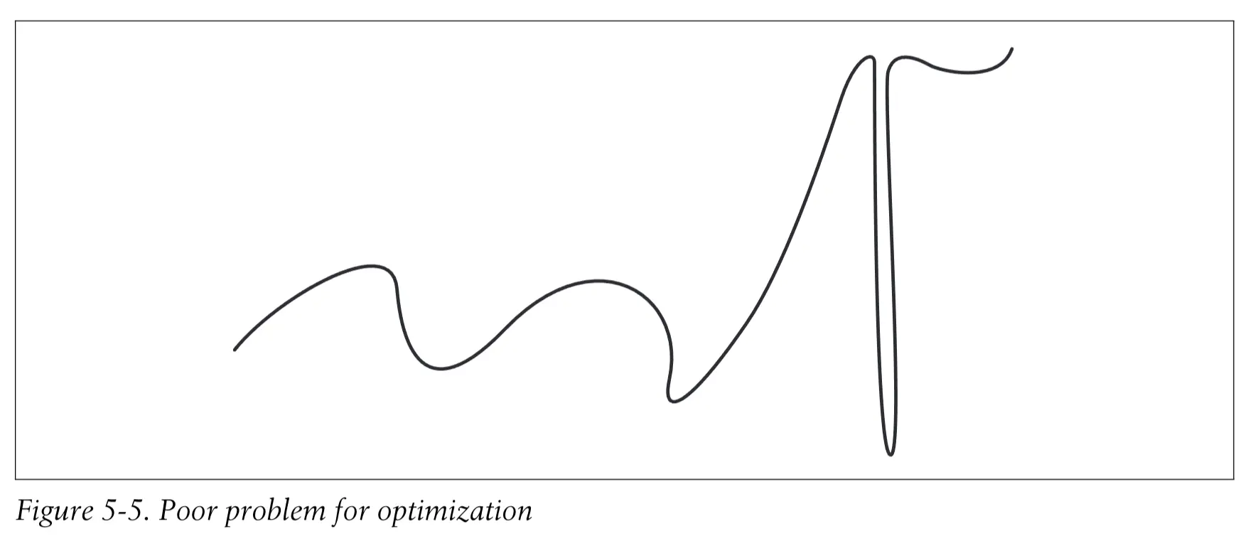
优化方式都有点取决于一个基本的事实
最优解应该接近于其他优解
如果有如下的一个例子就很难起效果
真实的航班搜索 #
网站已经更新了,这部分可以先 SKIP 了
偏好优化 #
学生宿舍优化问题 #
比如有 5 间宿舍,每个宿舍有 2 哥隔间,10 个学生来竞争居住,每个学生都有首选和次选,我们求一个最佳解
- 初始化代码
# The dorms, each of which has two available spaces
dorms=['Zeus','Athena','Hercules','Bacchus','Pluto']

# People, along with their first and second choices
prefs=[('Toby', ('Bacchus', 'Hercules')),
       ('Steve', ('Zeus', 'Pluto')),
       ('Karen', ('Athena', 'Zeus')),
       ('Sarah', ('Zeus', 'Pluto')),
       ('Dave', ('Athena', 'Bacchus')),
       ('Jeff', ('Hercules', 'Pluto')),
       ('Fred', ('Pluto', 'Athena')),
       ('Suzie', ('Bacchus', 'Hercules')),
       ('Laura', ('Bacchus', 'Hercules')),
       ('James', ('Hercules', 'Athena'))]
- 定义域
# 这里很巧妙,因为我们希望我们返回的都是有效解,这里的解比如
# [1,1,3,4,1,2,3,4,1,1] 也是一个有效解,是说,第一个人在剩余的里面选了 1,第二个是在剩余的里面选了 1,这样返回值应该永远有效
# [(0,9),(0,8),(0,7),(0,6),...,(0,0)]
domain=[(0,(len(dorms)*2)-i-1) for i in range(0,len(dorms)*2)]


def printsolution(vec):
  slots=[]
  # 创建一个结果集
  for i in range(len(dorms)): slots+=[i,i]

  # 遍历
  for i in range(len(vec)):
    x=int(vec[i])
    dorm=dorms[slots[x]]
    print prefs[i][0],dorm
    del slots[x]
- 定义成本函数
def dormcost(vec):
  cost=0
  # 创建一个槽位,每个槽位代表一个宿舍的一个隔间
  slots=[0,0,1,1,2,2,3,3,4,4]

  # 遍历结果,i 是 学生的下标
  for i in range(len(vec)):
    # 获取宿舍
    x=int(vec[i])
    # 找到这个宿舍
    dorm=dorms[slots[x]]
    # 找到这个学生的首选和次选
    pref=prefs[i][1]
    # 首选为 0
    # 次选为 1
    # 不在选择为 3
    if pref[0]==dorm: cost+=0
    elif pref[1]==dorm: cost+=1
    else: cost+=3

    # 删除选出来的,这样后面就不会再选到
    del slots[x]

  return cost
执行结果如下
s = optimization.geneticoptimize(domain,dormcost)
printsolution(s)

Toby Hercules
Steve Pluto
Karen Zeus
Sarah Zeus
Dave Athena
Jeff Pluto
Fred Athena
Suzie Bacchus
Laura Bacchus
James Hercules
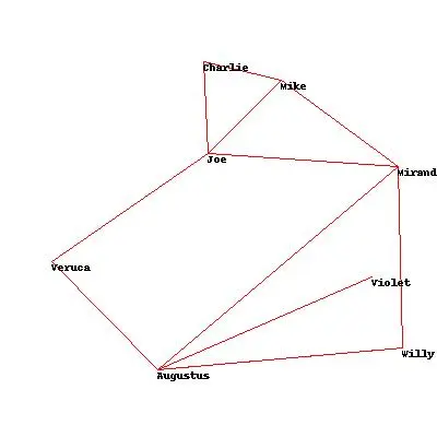
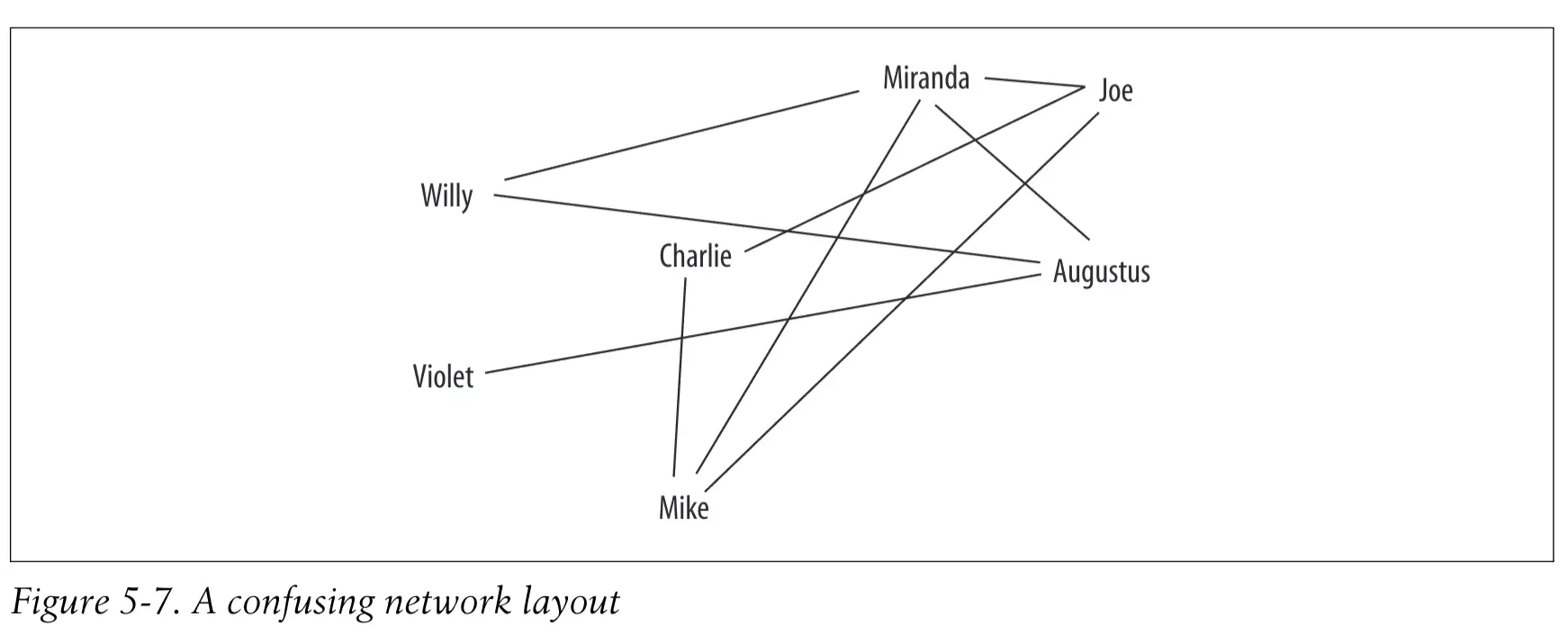
网络可视化 #
运用优化算法来构建更好的而非杂乱无章的网络图。
期望优化成如下
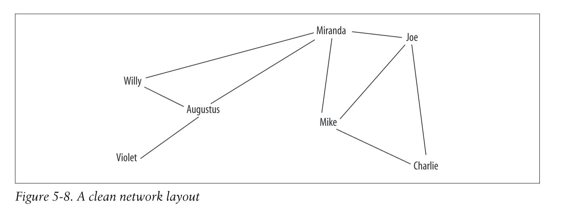
- 基础定义
people=['Charlie','Augustus','Veruca','Violet','Mike','Joe','Willy','Miranda']

links=[('Augustus', 'Willy'),
       ('Mike', 'Joe'),
       ('Miranda', 'Mike'),
       ('Violet', 'Augustus'),
       ('Miranda', 'Willy'),
       ('Charlie', 'Mike'),
       ('Veruca', 'Joe'),
       ('Miranda', 'Augustus'),
       ('Willy', 'Augustus'),
       ('Joe', 'Charlie'),
       ('Veruca', 'Augustus'),
       ('Miranda', 'Joe')]
想要图片变的好看,我们需要使用到 mass-and-spring 质点弹簧算法,
This type of algorithm is modeled on physicsbecause the different nodes exert a push on each other and try to move apart, whilethe links try to pull connected nodes closer together. 不同的点总是相互施加压力互相远离,而连线总是在缩短距离
- 定义成本函数
这里的成本函数就是如果交叉线越多,就是成本越高
结果可以用一个数组来表示
[120,30,200,125,....] 代表了 第一个人 在 (120,30) 的位置
def crosscount(v):
  # 数字序列转为人名的字典
  loc=dict([(people[i],(v[i*2],v[i*2+1])) for i in range(0,len(people))])
  total=0

  # 遍历所有的线
  for i in range(len(links)):
    for j in range(i+1,len(links)):

      # 获得坐标点
      (x1,y1),(x2,y2)=loc[links[i][0]],loc[links[i][1]]
      (x3,y3),(x4,y4)=loc[links[j][0]],loc[links[j][1]]

      den=(y4-y3)*(x2-x1)-(x4-x3)*(y2-y1)

      # 平行线就跳过
      if den==0: continue

      # 交叉线的分数
      ua=((x4-x3)*(y1-y3)-(y4-y3)*(x1-x3))/den
      ub=((x2-x1)*(y1-y3)-(y2-y1)*(x1-x3))/den

      # 交叉就是 +1
      if ua>0 and ua<1 and ub>0 and ub<1:
        total+=1

  return total
sol =optimization.randomoptimize(domain,costf=crosscount)
print crosscount(sol)

0
因为规模较小,还是很容易得到不交叉的结果
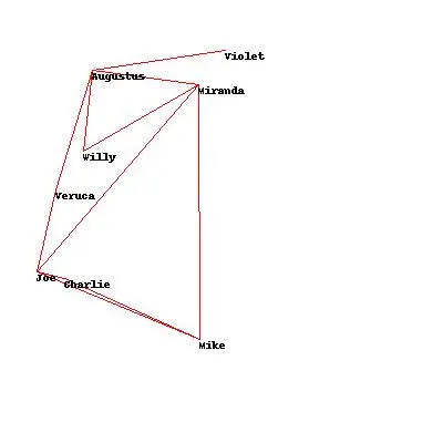
- 绘制图形
def drawnetwork(sol):
  img=Image.new('RGB',(400,400),(255,255,255))
  draw=ImageDraw.Draw(img)
  pos=dict([(people[i],(sol[i*2],sol[i*2+1])) for i in range(0,len(people))])

  for (a,b) in links:
    draw.line((pos[a],pos[b]),fill=(255,0,0))

  for n,p in pos.items():
    draw.text(p,n,(0,0,0))

  img.show()
默认生成的图片比较奇怪
- 更进步一步
我们可以在节点如果相近的情况下,增加分数,这样就会得到更好的结果
for i in range(len(people)):
  for j in range(i+1,len(people)):
    # 得到两个点
    (x1,y1),(x2,y2)=loc[people[i]],loc[people[j]]

    # 计算距离
    dist=math.sqrt(math.pow(x1-x2,2)+math.pow(y1-y2,2))
    # 太近了就扣分
    if dist<50:
      total+=(1.0-(dist/50.0))
现在生成的就会好一点